Node Settings
Last updated
Last updated
In this section, we will learn about each of the node properties in detail.
The node properties can be configured in the grid view as well as in the node settings panel.
In the grid view, click on the pencil icon next to the node name or click the Edit Node option from the toolbar to open the Node Settings window.
This window has 4 tabs as listed below.
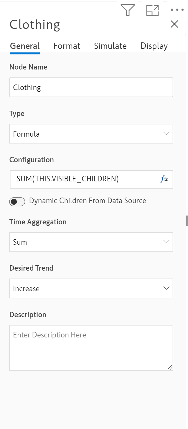
The General tab consists of some essential node properties such as Node Name, Type, Configuration, Time Aggregation, Desired Trend and Description.
Here, you can edit the name of the node.
The Type property is used to assign the nature of the node which helps in setting up the configuration. There are four node types to choose from.
Based on the Type selection, the configuration can be filled in as required by the user.
If the node is of formula type, the configuration can be filled in as a formula. You can manually type the formula or choose the required formula from the suggestions pop-up that appears as you start typing.
Note: Use Ctrl+Space to open all suggestions.
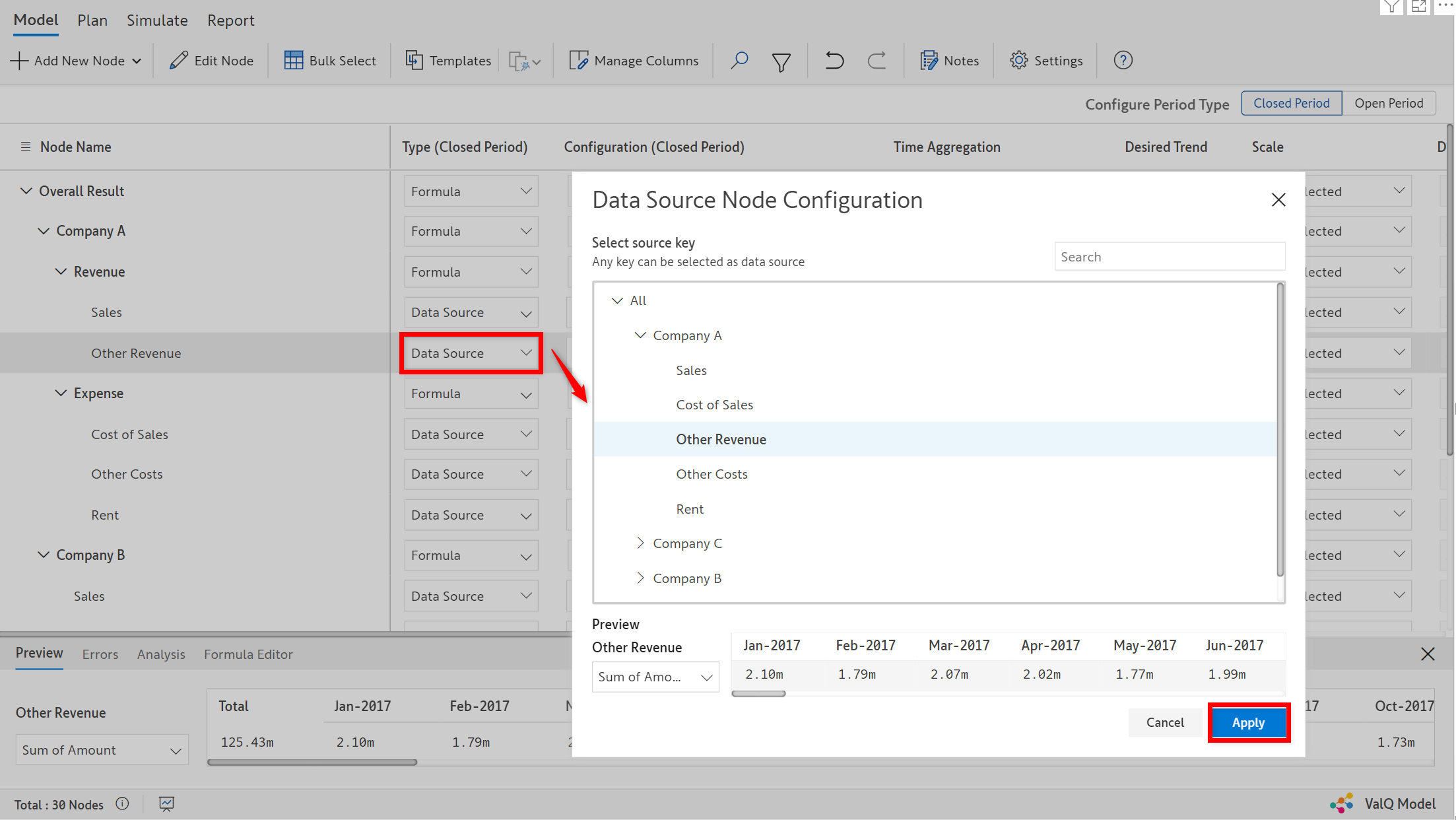
In this case, the node fetches the values from the source data based on the source key selected by the user.
This setting is used to instantly add all the descendant nodes from data, for Data Source nodes based on the selected source key. The nodes are identified from the Category Fields that are assigned to the visual.
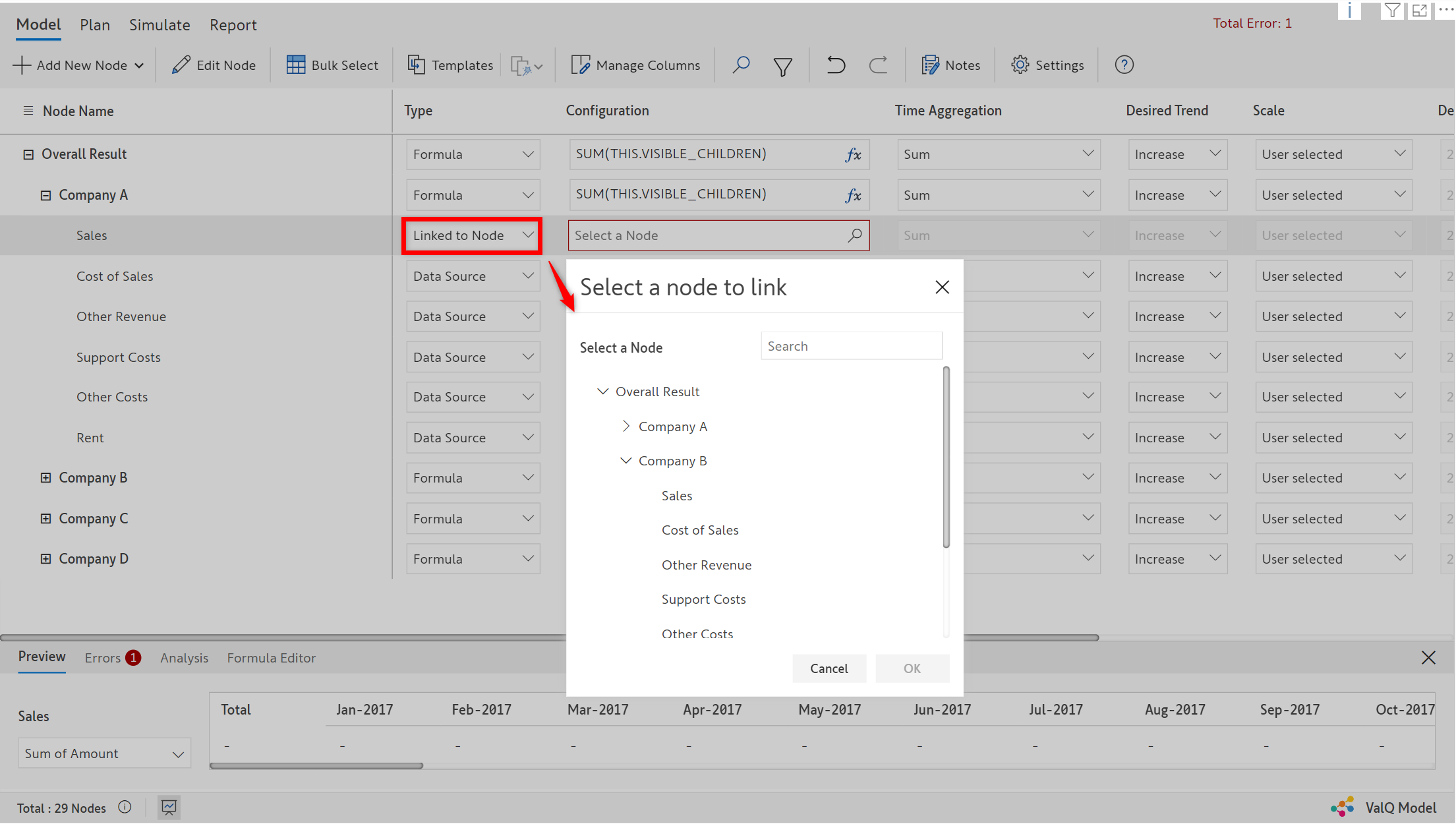
If the node type is ‘linked node’, then a node selection pop-up appears where you can choose a specific node to connect to.
Nodes that are linked share the same node value, properties, configuration, and simulation so that they mirror each other. Nodes are linked when the same node is required in many instances in the model.
For manual input-type nodes, users are allowed to fill in the node values manually.
In cases where you want to specify different node configurations for the open and the closed periods, you can enable hybrid configuration of nodes.
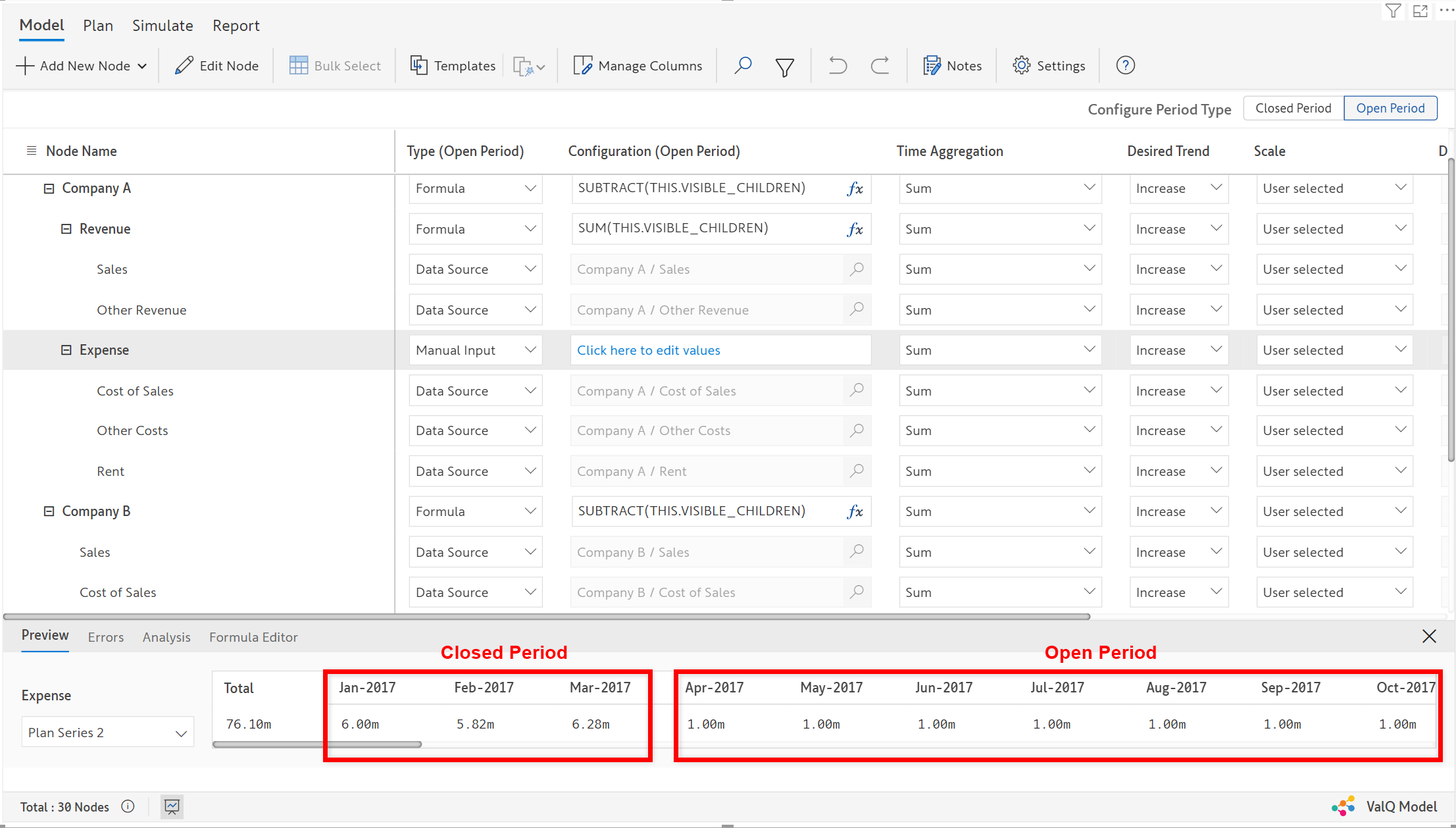
Open period values refer to the plan/forecast series and the closed period values refer to the actuals. Using this option, you can configure different formulas, data sources, or manual values for the actuals and the plan/forecast.
Hybrid configuration can be done only in editable models. For dynamic models, convert it to an editable one before configuring it for the open period.
The model looks as shown with an option to configure the nodes for the open period.
Convert the model to an editable model to start open period configuration.
The image below shows an example where the Expense node has two different configurations for the closed and open periods - formula type and manual input type respectively.
The node settings window also appears as shown below where you can configure the node for both open and closed periods.
The following example illustrates how the hybrid node configurations defined in the model are applied to the plan for the Expense node.
This property determines how the total node value needs to be calculated from its period values. The following are the different time aggregations available to the user.
The trend of the node can be set to Increase or Decrease depending on the context of the node. For instance, the Desired Trend for the Revenue node is Increase whereas for the Expense node, it is Decrease.
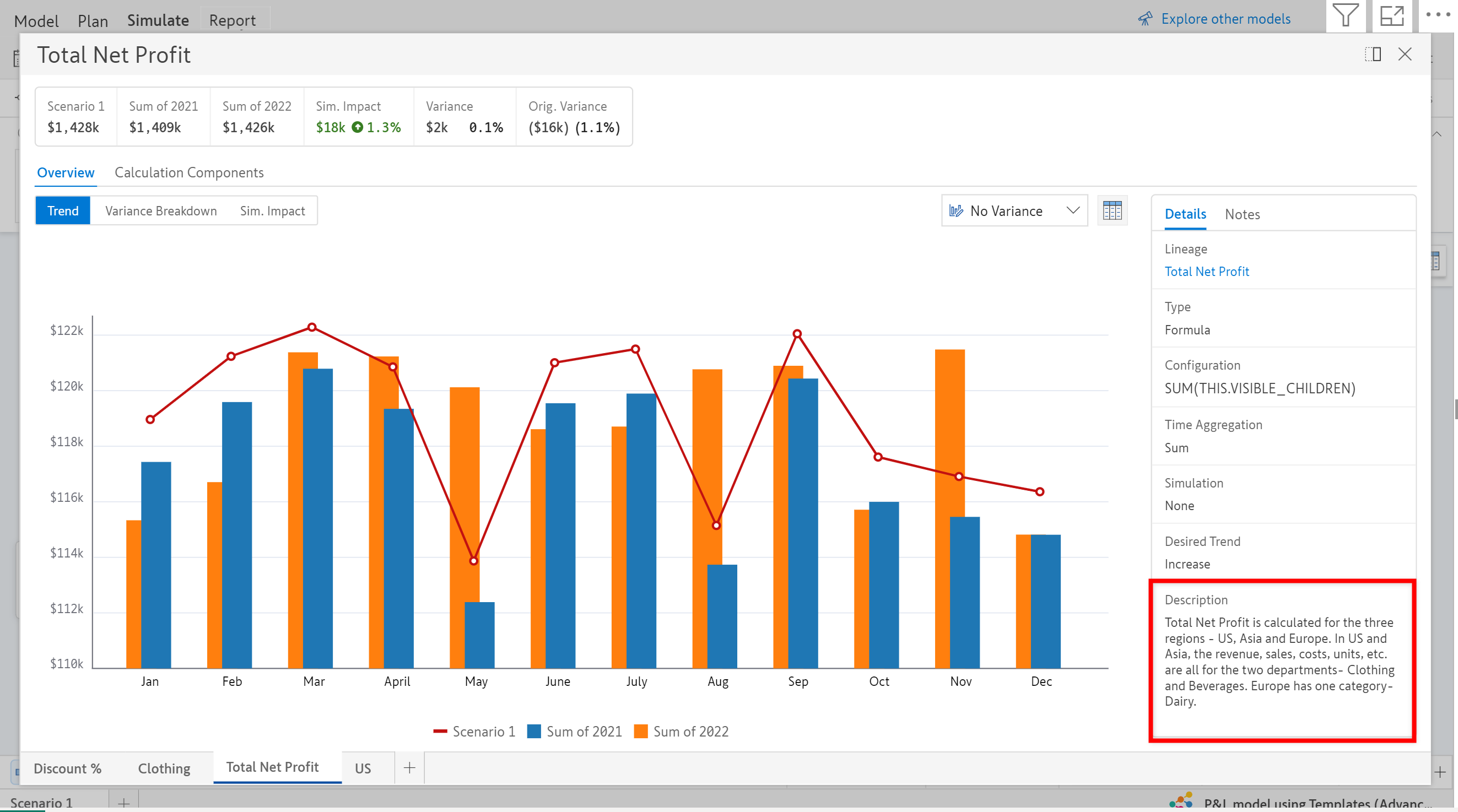
Any text describing the node or technical notes can be entered in the Description box.
The node description is also displayed in the respective node details screen on the Simulate tab.
The Format tab contains properties to edit the number formatting and conditional formatting of a node.
Under Number Formatting you can configure the scale, number of decimal places to display, prefix and suffix.
The User Selected option under Scale means that the scaling of the node is dynamic and gets changed when the user changes it on the Scaling Setting in the toolbar from any of the tabs.
Conditional Formatting can be used to configure the rules for the color formatting applied to the nodes on the Simulate tab. It can be applied based on the variance or the node value.
In the Simulate tab, you can configure simulation settings such as the Simulation Method and setting the slider's direction.
There are five methods by which simulation can be performed.
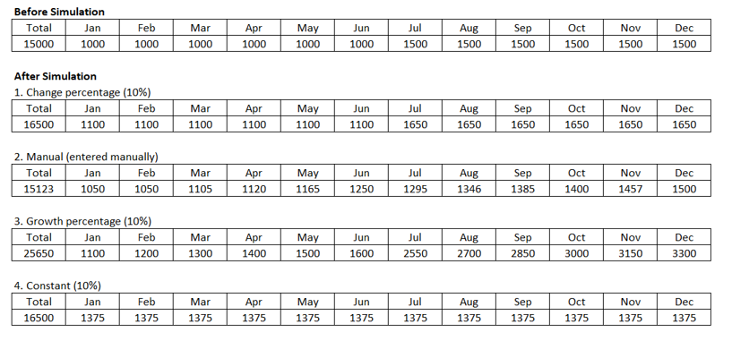
Change % - Percentage change applied to the baseline value.
Growth % - Percentage growth applied to the baseline value.
Constant - Constant value applied for all the simulation periods.
None - Disable simulation for the node.
Linked Simulation - Links the node's simulation to the selected node simulation (mirrors the simulation on it).
The simulation is always applied to the period values and the total node value is calculated depending on the node's Time Aggregation set by the user.
Here are the examples showing the node values before and after simulation under each method:
Slide Right to: To increase the node value on sliding right, set the Slide Right to property as Positive Simulation and to decrease the value set it as Negative Simulation.
Note: Simulation for dynamic children can be enabled or disabled at the top node in a dynamic model.
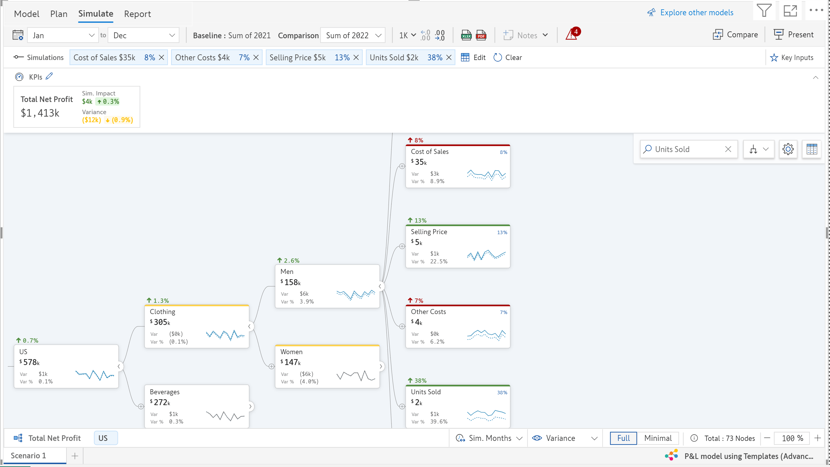
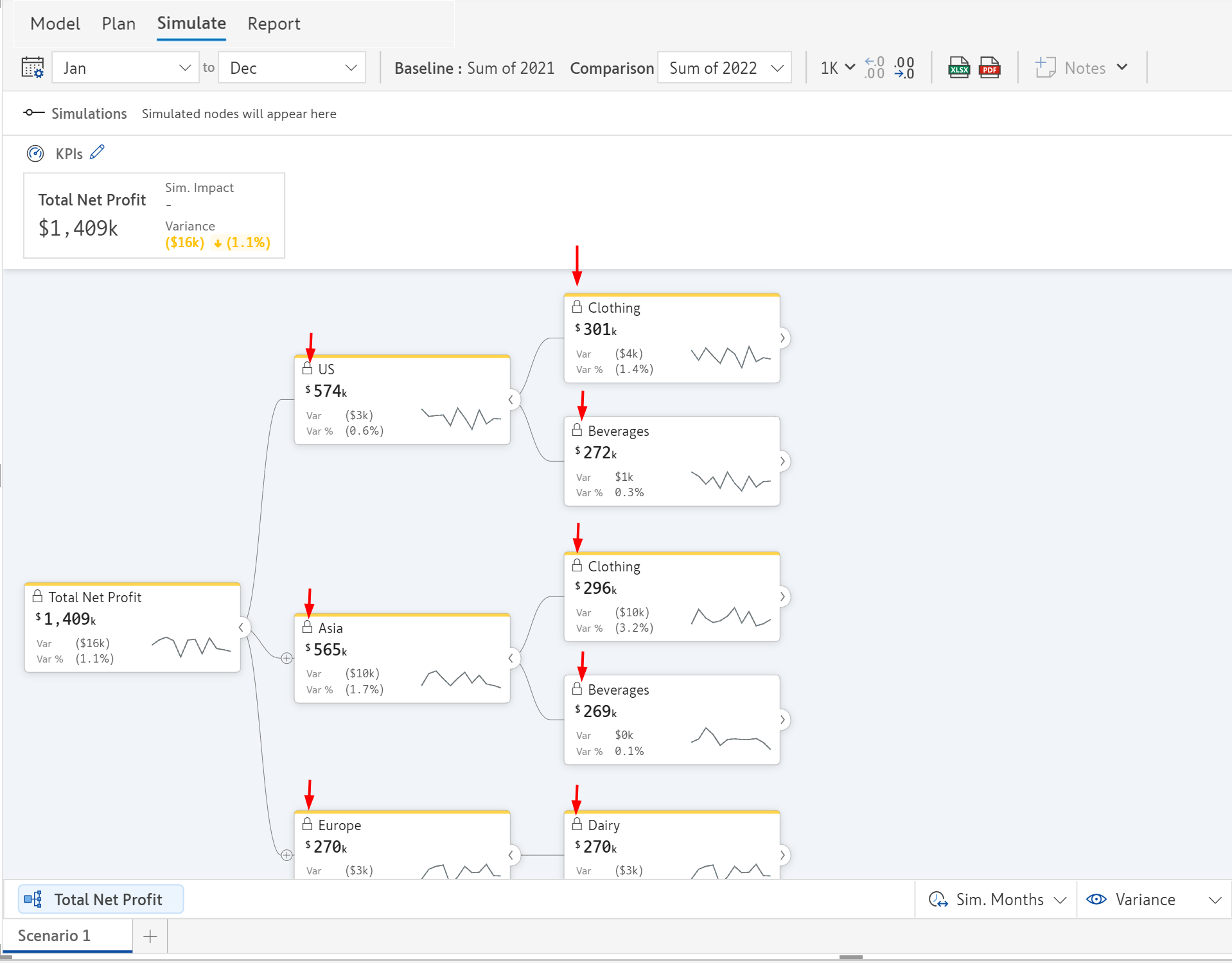
When the simulation is disabled, all data source nodes beneath the top node can not be simulated, as indicated by the simulation-disabled icon on the nodes.
You can toggle the same option to enable simulation - for all dynamic nodes or only the leaf nodes. The desired simulation method can also be selected for these nodes.
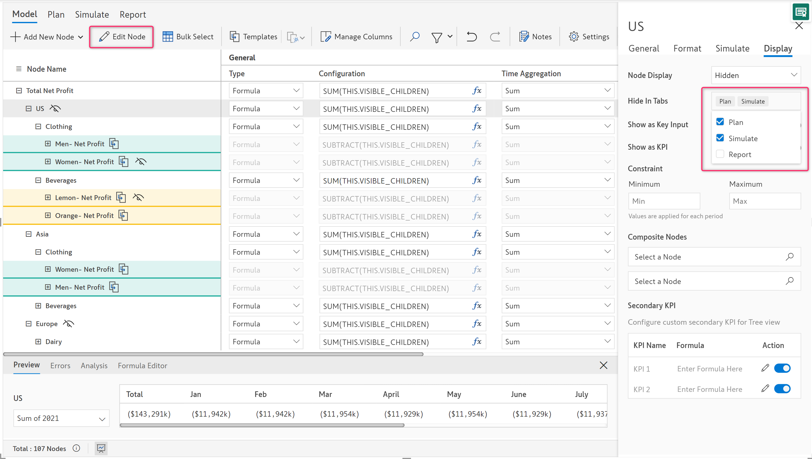
The Display tab is used to configure node settings such as node display, show as KPI or Key Input, setting up constraints, adding composite nodes and customizing secondary KPI.
The display settings configured here (except the Node Display option) apply to the Simulate tab, i.e. any changes made here would reflect on the Simulate tab.
This property determines whether the node should appear on the model and how it should appear. It changes the node's visibility across the other tabs, while the nodes are always available in the Model tab for configuration. The Node Display dropdown consists of the following three options:
Show - Displays the node as a normal node (Default).
Derived - Displays the node as being derived from its parent. It is denoted by a dotted line and transparent node tile in the Simulate tab - tree view.
Hidden - The node is hidden from the visual based on the tabs chosen, but it is available for calculation and other references in the Model tab. If a parent node is hidden all the descendants under it also get hidden.
This dropdown menu appears when you choose the Hidden option in the Node Display to hide a node. You can select the tabs where you want the node to be hidden.
Node Display of the root node can never be set as Derived or Hidden.
To add/show the node as a key input in the Key Inputs section or as a KPI in the KPI ribbon on the Simulate tab, enable any of these toggle buttons.
Constraint can be added to a node by way of assigning minimum and maximum threshold values a node can have, against which you can evaluate the model's performance.
To set a constraint for a node, go to the Constraint section in the Display tab. Then enter the minimum and maximum values permissible for that node.
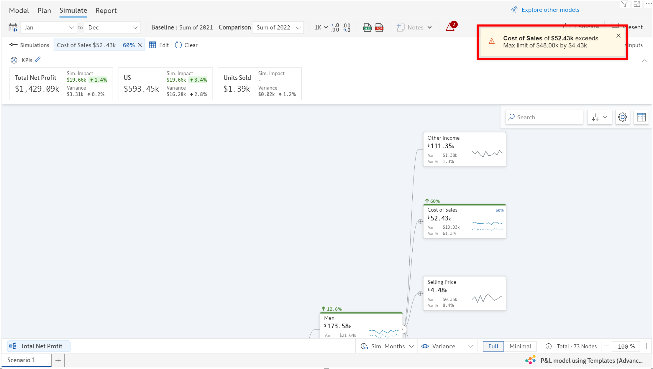
In the below example, the constraint for Cost of Sales is set with the minimum and maximum values as 2700 and 4000 respectively.
The values entered are for each period and hence the minimum and maximum limits for that node are computed as the product of the value entered and the number of periods. As there are 12 periods available here, 12 * 2700 and 12 * 4000 are the limits. Therefore, the minimum and maximum threshold values would be 32400 and 48000 respectively.
If the cost of sales exceeds $48000 or falls below $32400 in any scenario during simulation, a warning is displayed to the user about the constraint along with the difference in value by which the simulated result exceeds or falls below the threshold levels.
Click on the warning symbol to view all the constraints violated in the model.
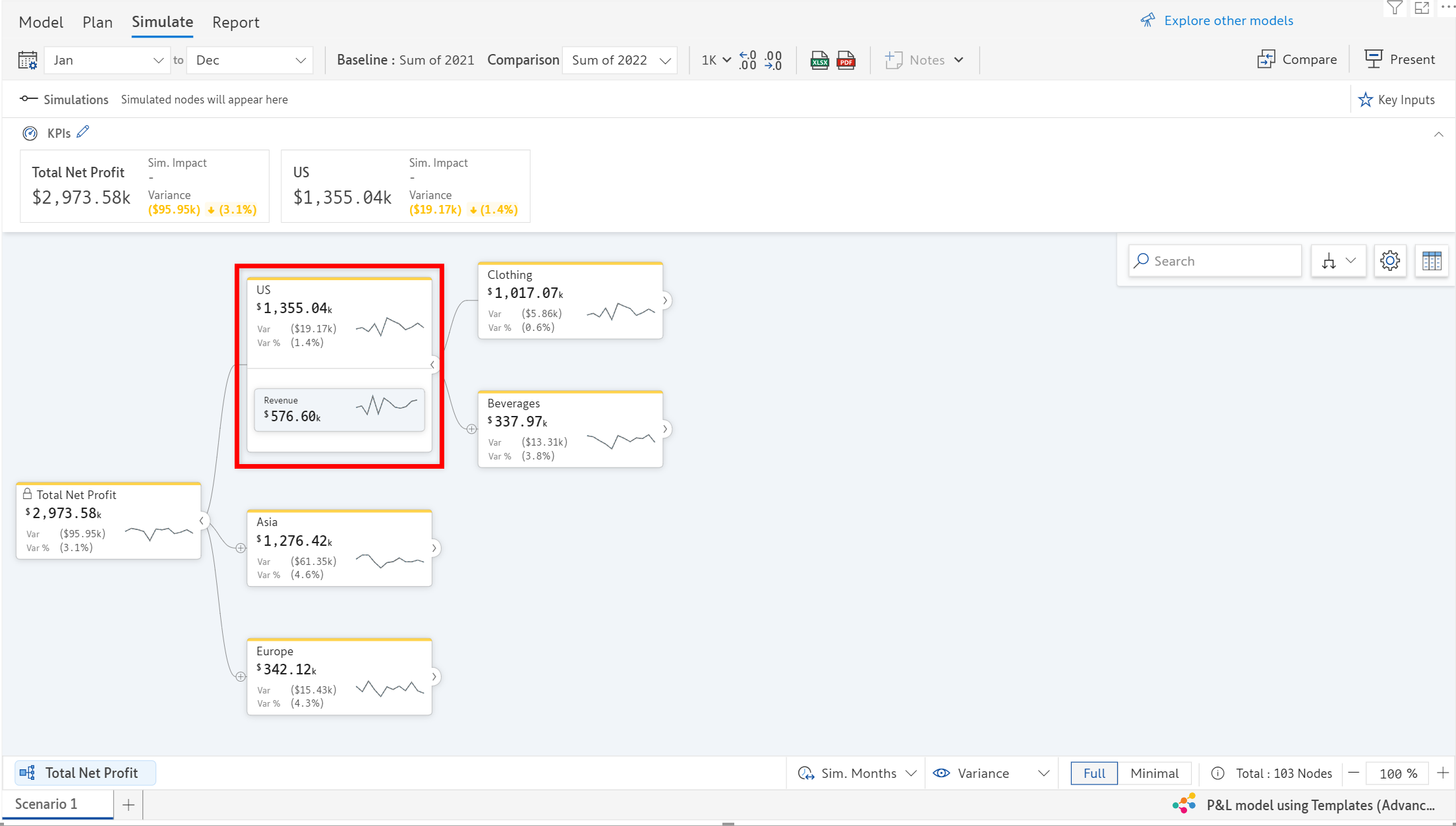
When there is a large number of nodes in the model, and you want to take a quick look at another node that is important along with the current node you can use the Composite Nodes option. This option helps you to include up to two nodes within the node's tile that are important or relevant to it.
To add a composite node, click Select a node, choose the node you want to add and click OK.
In the Simulate tab, it appears as shown below. Revenue node is added to US node so that you can have a quick look at Revenue and also simulate it.
The composite nodes option is for the visual arrangement of nodes and does not impact their relationship or the dependency of nodes.
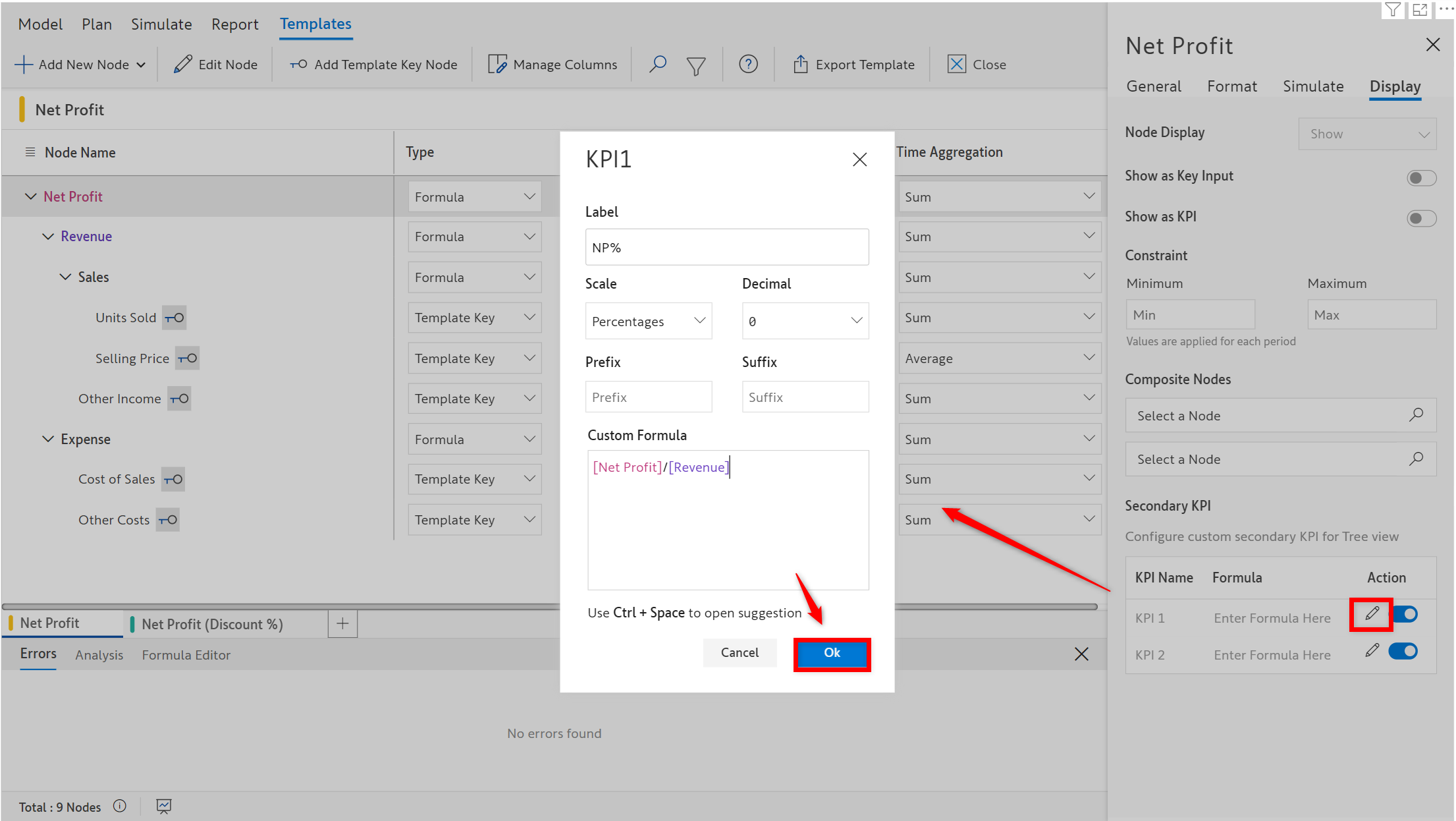
Secondary KPI helps you to insert additional values to the node tile. Under this property, you can input up to 2 customized secondary KPI values to the node tile.
In the below example, Net Profit Margin is to be added as a secondary KPI to all Net Profit nodes. Since these are template nodes, go to Templates Sections and click on the Edit Node option for the Net Profit node in the template available.
Go to Secondary KPI in the Display section and click on the pencil icon. Enter the formula/function you want as the Secondary KPI, enter a label for it and click OK.
For more help on the usage of different formulas and functions, you can refer to .
For a model that contains templates, use the Templates window to include open-period configuration for the template nodes. Templates are covered in detail in the .
To enable open period node configuration, toggle the button below in the window.
Formula
ValQ computes and executes the user-defined formula on the node.
Data Source
The node gets the values directly from the source data.
Linked to Node
The node value, its properties and simulation are linked to another node.
Manual Input
The user can enter the values manually for this type of node.
Sum
Adds all the period values
Average
Calculates the average of the period values
Average Excluding Zeros
Calculates the average of the non-zero period values
Formula
Calculates and applies the custom formula entered by the user
Last
Only displays the last period value of the node
Running Total
Cumulative total of the period values of the node
Weighted Average
Calculates the weighted average of the period values based on the nodes from which the weights are taken.